Skip to content

Open In Colab

Setup

This is the Google colab version of the Monocle 2 notebook on the kallisto | bustools R notebook website. This version follows the static version closely, but uses the 10xv3 1k E18 mouse neuron dataset to reduce download time and runtime for interactive use here. Google colab gives each notebook a fresh Ubuntu machine with R and some common packages pre-installed. Here we install the packages used in the downstream analysis that are not pre-installed. This takes a while, as some of the packages have several dependencies that have C++ code; it seems that most of time spent installing these packages is spent on compiling C++ code. Package installation might not have taken this long in your experience, since you most likely already have many of the common dependencies installed on your computer, which is not the case here.

1
2
install.packages("BiocManager")
BiocManager::install(c("DropletUtils", "monocle", "SingleR", "BUSpaRse", "scater", "scran"))
Installing package into /usr/local/lib/R/site-library
(as lib is unspecified)

Bioconductor version 3.10 (BiocManager 1.30.10), R 3.6.2 (2019-12-12)

Installing package(s) 'BiocVersion', 'DropletUtils', 'monocle', 'SingleR',
  'BUSpaRse'

also installing the dependencies formatR, bit, vctrs, lambda.r, futile.options, bitops, interactiveDisplayBase, bit64, blob, DBI, zlibbioc, Rhtslib, futile.logger, snow, locfit, IRanges, R.oo, R.methodsS3, sitmo, RcppEigen, FNN, ggrepel, gridExtra, sparsesvd, docopt, graph, RBGL, XML, RCurl, RUnit, RcppAnnoy, RcppHNSW, AnnotationHub, BiocFileCache, rappdirs, RSQLite, XVector, rtracklayer, Rsamtools, ProtGenerics, GenomeInfoDbData, GenomicAlignments, SingleCellExperiment, S4Vectors, BiocParallel, edgeR, rhdf5, HDF5Array, R.utils, dqrng, beachmat, Rhdf5lib, Biobase, VGAM, DDRTree, igraph, BiocGenerics, HSMMSingleCell, combinat, fastICA, irlba, matrixStats, densityClust, Rtsne, limma, qlcMatrix, pheatmap, proxy, slam, viridis, biocViews, RANN, SummarizedExperiment, DelayedArray, DelayedMatrixStats, BiocNeighbors, ExperimentHub, AnnotationDbi, AnnotationFilter, biomaRt, Biostrings, BSgenome, data.table, ensembldb, GenomeInfoDb, GenomicFeatures, GenomicRanges, plyranges, RcppParallel, RcppArmadillo, RcppProgress


Old packages: 'BH', 'broom', 'callr', 'cli', 'curl', 'DBI', 'DT', 'fansi',
  'farver', 'gh', 'hms', 'knitr', 'mime', 'pillar', 'prettyunits', 'rlang',
  'rmarkdown', 'rprojroot', 'stringi', 'tidyr', 'tinytex', 'vctrs', 'xfun',
  'xtable', 'boot', 'foreign', 'MASS'
1
2
3
system("wget https://github.com/pachterlab/kallisto/releases/download/v0.46.1/kallisto_linux-v0.46.1.tar.gz")
untar("kallisto_linux-v0.46.1.tar.gz")
system("cp kallisto/kallisto /usr/local/bin")

To get from fastq files to the gene count matrix, we will use the kb wrapper of kallisto and bustools here, which condenses several commands directly calling kallisto and bustools into 2. See the static version of this notebook for instructions of calling kallisto and bustools directly.

1
system("pip3 install kb-python")
1
2
3
4
5
6
7
8
library(BUSpaRse)
library(DropletUtils)
library(scater)
library(monocle)
library(SingleR)
library(Matrix)
library(tidyverse)
theme_set(theme_bw())
Loading required package: SingleCellExperiment

Loading required package: SummarizedExperiment

Loading required package: GenomicRanges

Loading required package: stats4

Loading required package: BiocGenerics

Loading required package: parallel


Attaching package: 'BiocGenerics'


The following objects are masked from 'package:parallel':

    clusterApply, clusterApplyLB, clusterCall, clusterEvalQ,
    clusterExport, clusterMap, parApply, parCapply, parLapply,
    parLapplyLB, parRapply, parSapply, parSapplyLB


The following objects are masked from 'package:stats':

    IQR, mad, sd, var, xtabs


The following objects are masked from 'package:base':

    anyDuplicated, append, as.data.frame, basename, cbind, colnames,
    dirname, do.call, duplicated, eval, evalq, Filter, Find, get, grep,
    grepl, intersect, is.unsorted, lapply, Map, mapply, match, mget,
    order, paste, pmax, pmax.int, pmin, pmin.int, Position, rank,
    rbind, Reduce, rownames, sapply, setdiff, sort, table, tapply,
    union, unique, unsplit, which, which.max, which.min


Loading required package: S4Vectors


Attaching package: 'S4Vectors'


The following object is masked from 'package:base':

    expand.grid


Loading required package: IRanges

Loading required package: GenomeInfoDb

Loading required package: Biobase

Welcome to Bioconductor

    Vignettes contain introductory material; view with
    'browseVignettes()'. To cite Bioconductor, see
    'citation("Biobase")', and for packages 'citation("pkgname")'.


Loading required package: DelayedArray

Loading required package: matrixStats


Attaching package: 'matrixStats'


The following objects are masked from 'package:Biobase':

    anyMissing, rowMedians


Loading required package: BiocParallel


Attaching package: 'DelayedArray'


The following objects are masked from 'package:matrixStats':

    colMaxs, colMins, colRanges, rowMaxs, rowMins, rowRanges


The following objects are masked from 'package:base':

    aperm, apply, rowsum


Loading required package: ggplot2

Loading required package: Matrix


Attaching package: 'Matrix'


The following object is masked from 'package:S4Vectors':

    expand


Loading required package: VGAM

Loading required package: splines

Loading required package: DDRTree

Loading required package: irlba

── Attaching packages ─────────────────────────────────────── tidyverse 1.3.0 ──

✔ tibble  2.1.3     ✔ dplyr   0.8.3
✔ tidyr   1.0.0     ✔ stringr 1.4.0
✔ readr   1.3.1     ✔ forcats 0.4.0
✔ purrr   0.3.3

── Conflicts ────────────────────────────────────────── tidyverse_conflicts() ──
✖ dplyr::collapse()   masks IRanges::collapse()
✖ dplyr::combine()    masks Biobase::combine(), BiocGenerics::combine()
✖ dplyr::count()      masks matrixStats::count()
✖ dplyr::desc()       masks IRanges::desc()
✖ tidyr::expand()     masks Matrix::expand(), S4Vectors::expand()
✖ tidyr::fill()       masks VGAM::fill()
✖ dplyr::filter()     masks stats::filter()
✖ dplyr::first()      masks S4Vectors::first()
✖ dplyr::lag()        masks stats::lag()
✖ tidyr::pack()       masks Matrix::pack()
✖ ggplot2::Position() masks BiocGenerics::Position(), base::Position()
✖ purrr::reduce()     masks GenomicRanges::reduce(), IRanges::reduce()
✖ dplyr::rename()     masks S4Vectors::rename()
✖ purrr::simplify()   masks DelayedArray::simplify()
✖ dplyr::slice()      masks IRanges::slice()
✖ tidyr::unpack()     masks Matrix::unpack()

Download data

1
2
3
4
5
6
# Download data
if (!dir.exists("./data")) dir.create("./data")
if (!file.exists("./data/neuron_1k_v3_fastqs.tar")) {
  download.file("http://cf.10xgenomics.com/samples/cell-exp/3.0.0/neuron_1k_v3/neuron_1k_v3_fastqs.tar", 
      "./data/neuron_1k_v3_fastqs.tar", method = "wget", quiet = TRUE)
}
1
untar("./data/neuron_1k_v3_fastqs.tar", exdir = "./data")

Generate the gene count matrix

Build the kallisto index

Here we use kallisto to pseudoalign the reads to the transcriptome and then to create the bus file to be converted to a sparse matrix. The first step is to build an index of the mouse transcriptome. The transcriptome downloaded here is Ensembl version 99, the most recent version as of writing.

1
2
3
4
5
6
# Mouse transcriptome
if (!dir.exists("./reference")) dir.create("./reference")
if (!file.exists("./reference/mm_cdna99.fa.gz")) {
  download.file("ftp://ftp.ensembl.org/pub/release-99/fasta/mus_musculus/cdna/Mus_musculus.GRCm38.cdna.all.fa.gz", 
  "./reference/mm_cdna99.fa.gz", method = "wget", quiet = TRUE)
}
1
system("kallisto index -i ./reference/mm_tr_index99.idx ./reference/mm_cdna99.fa.gz", intern = TRUE)

Map transcripts to genes

For the sparse matrix, most people are interested in how many UMIs per gene per cell, we here we will quantify this from the bus output, and to do so, we need to find which gene corresponds to each transcript. Remember in the output of kallisto bus, there's the file transcripts.txt. Those are the transcripts in the transcriptome index.

Remember that we downloaded transcriptome FASTA file from Ensembl just now. In FASTA files, each entry is a sequence with a name. In Ensembl FASTA files, the sequence name has genome annotation of the corresponding sequence, so we can extract transcript IDs and corresponding gene IDs and gene names from there.

1
tr2g <- tr2g_fasta("./reference/mm_cdna99.fa.gz")
Reading FASTA file.
1
head(tr2g)
A tibble: 6 × 3
transcriptgenegene_name
<chr><chr><chr>
ENSMUST00000177564.1ENSMUSG00000096176.1Trdd2
ENSMUST00000196221.1ENSMUSG00000096749.2Trdd1
ENSMUST00000179664.1ENSMUSG00000096749.2Trdd1
ENSMUST00000178537.1ENSMUSG00000095668.1Trbd1
ENSMUST00000178862.1ENSMUSG00000094569.1Trbd2
ENSMUST00000179520.1ENSMUSG00000094028.1Ighd4-1

bustools requires tr2g to be written into a tab delimited file of a specific format: No headers, first column is transcript ID, and second column is the corresponding gene ID. Transcript IDs must be in the same order as in the kallisto index.

1
2
# Write tr2g to format required by bustools
save_tr2g_bustools(tr2g, file_save = "./reference/tr2g_mm99.tsv")

Using the kb wrapper

With kallisto and bustools, it takes several commands to go from fastq files to the spliced and unspliced matrices, which is quite cumbersome. So a wrapper called kb was written to condense those steps to one. The command line tool kb can be installed with

Then we can use the following command to generate the spliced and unspliced matrices:

1
system("chmod -R 777 data/")
1
2
3
fn <- list.files("data/neuron_1k_v3_fastqs", full.names = TRUE)
fn <- fn[str_detect(fn, "R\\d_")]
fn
  1. 'data/neuron_1k_v3_fastqs/neuron_1k_v3_S1_L001_R1_001.fastq.gz'
  2. 'data/neuron_1k_v3_fastqs/neuron_1k_v3_S1_L001_R2_001.fastq.gz'
  3. 'data/neuron_1k_v3_fastqs/neuron_1k_v3_S1_L002_R1_001.fastq.gz'
  4. 'data/neuron_1k_v3_fastqs/neuron_1k_v3_S1_L002_R2_001.fastq.gz'
1
2
system(paste("kb count -i reference/mm_tr_index99.idx -g reference/tr2g_mm99.tsv -x 10xv3 -o output",
paste(fn, collapse = " ")), intern = TRUE)

Preprocessing

Now we can load the matrix into R for analysis.

1
res_mat <- read_count_output("./output/counts_unfiltered", name = "cells_x_genes", tcc = FALSE)

Remove empty droplets

1
dim(res_mat)
  1. 36711
  2. 399524

The number of genes seems reasonable. The number of barcodes is way larger than the expected ~10k.

1
2
tot_counts <- Matrix::colSums(res_mat)
summary(tot_counts)
     Min.   1st Qu.    Median      Mean   3rd Qu.      Max. 
     0.00      1.00      1.00     40.47      5.00 154216.00

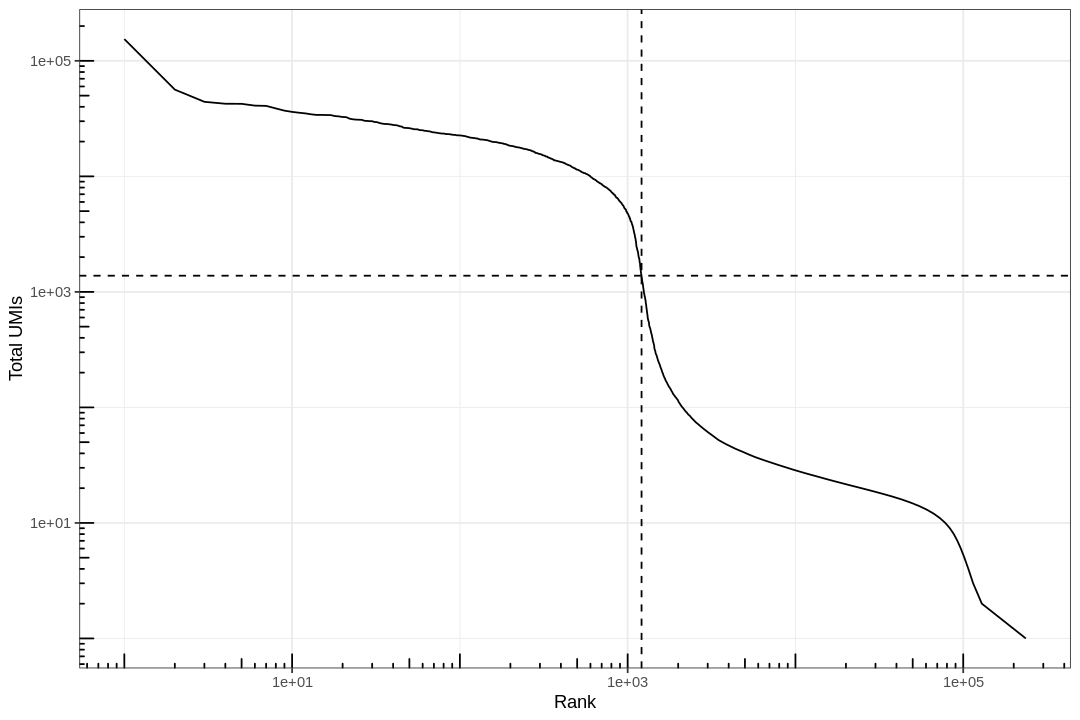
The vast majority of "cells" have only no or just a few UMI detected. Those are empty droplets. 10x claims to have cell capture rate of up to 65%, but in practice, depending on how many cells are in fact loaded, the rate can be much lower. A commonly used method to estimate the number of empty droplets is barcode ranking knee and inflection points, as those are often assumed to represent transition between two components of a distribution. While more sophisticated methods exist (e.g. see emptyDrops in DropletUtils), for simplicity, we will use the barcode ranking method here. However, whichever way we go, we don't have the ground truth.

1
2
# Compute barcode rank
bc_rank <- barcodeRanks(res_mat, lower = 1000)
 1
 2
 3
 4
 5
 6
 7
 8
 9
10
11
12
13
14
15
16
17
18
19
20
21
22
23
24
25
#' Knee plot for filtering empty droplets
#' 
#' Visualizes the inflection point to filter empty droplets. This function plots 
#' different datasets with a different color. Facets can be added after calling
#' this function with `facet_*` functions.
#' 
#' @param bc_rank A `DataFrame` output from `DropletUtil::barcodeRanks`.
#' @return A ggplot2 object.
knee_plot <- function(bc_rank) {
  knee_plt <- tibble(rank = bc_rank[["rank"]],
                     total = bc_rank[["total"]]) %>% 
    distinct() %>% 
    dplyr::filter(total > 0)
  annot <- tibble(inflection = metadata(bc_rank)[["inflection"]],
                  rank_cutoff = max(bc_rank$rank[bc_rank$total > metadata(bc_rank)[["inflection"]]]))
  p <- ggplot(knee_plt, aes(rank, total)) +
    geom_line() +
    geom_hline(aes(yintercept = inflection), data = annot, linetype = 2) +
    geom_vline(aes(xintercept = rank_cutoff), data = annot, linetype = 2) +
    scale_x_log10() +
    scale_y_log10() +
    annotation_logticks() +
    labs(x = "Rank", y = "Total UMIs")
  return(p)
}
1
2
options(repr.plot.width=9, repr.plot.height=6)
knee_plot(bc_rank)

png

1
2
3
4
# Filter the matrix
res_mat <- res_mat[, tot_counts > metadata(bc_rank)$inflection]
res_mat <- res_mat[Matrix::rowSums(res_mat) > 0,]
dim(res_mat)
  1. 20198
  2. 1210
1
rownames(res_mat) <- str_remove(rownames(res_mat), "\\.\\d+")

Now the number of cells is closer to expectation.

Cell type inference

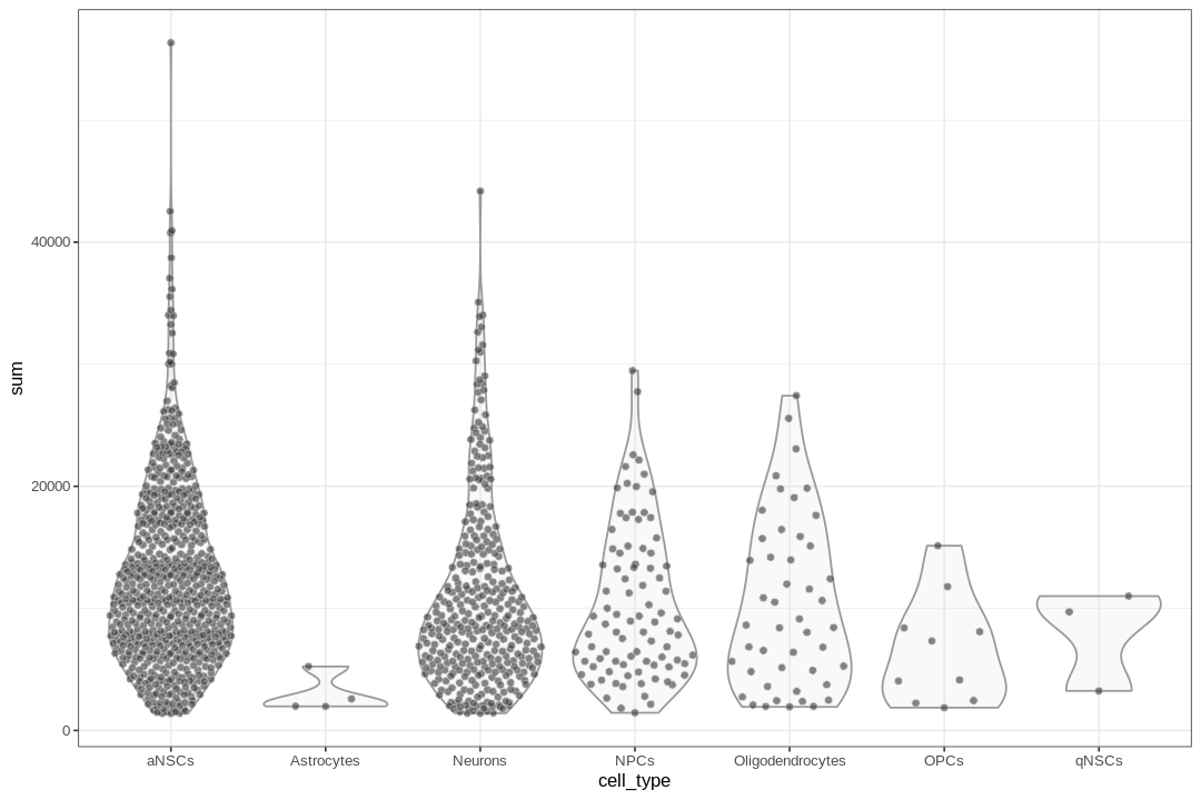
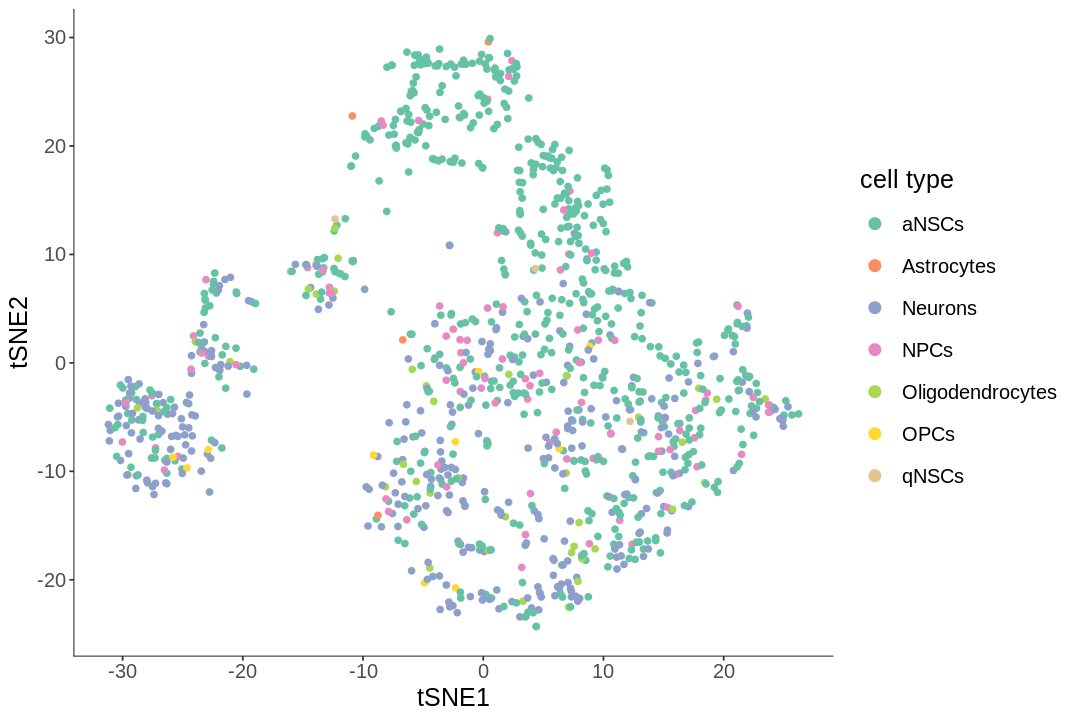
Monocle 2 only infers one trajectory for the entire dataset, so non-neuronal cells like endothelial cells and erythrocytes may be mistaken as highly differentiated cells from the neuronal lineage. So we will remove cell types not of the neural or glial lineages. Cell types are also helpful to orient the trajectory; neuronal progenitor cells must come before neurons. Here cell type inference is done programatically with SingleR, which compares gene expression profiles of individual cells to bulk RNA-seq data of purified known cell types.

1
2
3
mouse.rnaseq <- MouseRNAseqData(ensembl = TRUE)
sce <- SingleCellExperiment(assays = list(counts = res_mat))
sce <- logNormCounts(sce)

Then SingleR will assign each cell a label based on Spearman correlation with known cell types from bulk RNA-seq. These are meanings of the acronyms:

  • OPCs: Oligodendrocyte progenitor cells
  • NPCs: Neural progenitor cells
  • aNSCs: Active neural stem cells
  • qNSCs: Quiescent neural stem cells
1
2
annots <- SingleR(sce, ref = mouse.rnaseq, labels = colData(mouse.rnaseq)$label.fine,
de.method = "wilcox", method = "single", BPPARAM = MulticoreParam(4))
1
annots
DataFrame with 1210 rows and 5 columns
                                                                        scores
                                                                      <matrix>
AAACGCTGTAATGTGA    0.0601901483760862:0.242986808015721:0.177660752587073:...
AAACGCTGTCCTGGGT      0.11153546550616:0.321858508786419:0.206383027494298:...
AAAGAACCAGGACATG    0.0585569289411892:0.225038532259566:0.177381655702582:...
AAAGGTACACACGGTC       0.137923692580242:0.3506611435018:0.281933499704427:...
AAAGGTATCACCATAG -0.00511350381259525:0.166880227412372:0.0975899954539976:...
...                                                                        ...
TTTGACTTCGTTCAGA     0.100933655338997:0.327948884202836:0.262011719832591:...
TTTGATCTCCATAGGT     0.0656536744266451:0.280702755051776:0.23375860874247:...
TTTGGAGAGGCTAACG    0.0681422805975054:0.234772340818692:0.176292333613646:...
TTTGGTTAGTAATCCC     0.125780004617712:0.315213344287222:0.258722018820061:...
TTTGTTGGTATGGAAT    0.0512710432754663:0.231028330364938:0.177598025280379:...
                 first.labels                        tuning.scores      labels
                  <character>                          <DataFrame> <character>
AAACGCTGTAATGTGA        aNSCs  0.233804530306167:0.219682141602258       aNSCs
AAACGCTGTCCTGGGT         NPCs                                  1:1       aNSCs
AAAGAACCAGGACATG      Neurons                                  1:1       aNSCs
AAAGGTACACACGGTC         NPCs                                  1:1       aNSCs
AAAGGTATCACCATAG         NPCs                              0.5:0.5       aNSCs
...                       ...                                  ...         ...
TTTGACTTCGTTCAGA      Neurons                                  1:1       aNSCs
TTTGATCTCCATAGGT      Neurons                              0.5:0.5       aNSCs
TTTGGAGAGGCTAACG        aNSCs 0.209611614011623:0.0580258853185659     Neurons
TTTGGTTAGTAATCCC      Neurons 0.187703782257732:-0.195976600339204     Neurons
TTTGTTGGTATGGAAT         OPCs 0.299839391397521:-0.199361864824359     Neurons
                 pruned.labels
                   <character>
AAACGCTGTAATGTGA         aNSCs
AAACGCTGTCCTGGGT         aNSCs
AAAGAACCAGGACATG         aNSCs
AAAGGTACACACGGTC         aNSCs
AAAGGTATCACCATAG         aNSCs
...                        ...
TTTGACTTCGTTCAGA         aNSCs
TTTGATCTCCATAGGT         aNSCs
TTTGGAGAGGCTAACG       Neurons
TTTGGTTAGTAATCCC       Neurons
TTTGTTGGTATGGAAT       Neurons
1
2
3
4
5
6
inds <- annots$pruned.labels %in% c("NPCs", "Neurons", "OPCs", "Oligodendrocytes", 
                                    "qNSCs", "aNSCs", "Astrocytes", "Ependymal")
# Only keep these cell types
cells_use <- row.names(annots)[inds]
sce <- sce[, cells_use]
sce$cell_type <- annots$pruned.labels[inds]

QC

1
df <- perCellQCMetrics(sce)
1
colData(sce) <- cbind(colData(sce), df)
1
colData(sce)
DataFrame with 1146 rows and 8 columns
                   cell_type       sum  detected   percent_top_50
                 <character> <numeric> <integer>        <numeric>
AAACGCTGTAATGTGA       aNSCs      7072      3256 19.0328054298643
AAACGCTGTCCTGGGT       aNSCs      9458      4101 12.8991330090928
AAAGAACCAGGACATG       aNSCs      5338      2577 20.7006369426752
AAAGGTACACACGGTC       aNSCs     16892      5111 18.2098034572579
AAAGGTATCACCATAG       aNSCs      1397       882 24.9105225483178
...                      ...       ...       ...              ...
TTTGACTTCGTTCAGA       aNSCs     26203      6091 21.4021295271534
TTTGATCTCCATAGGT       aNSCs      8120      3625 16.7980295566502
TTTGGAGAGGCTAACG     Neurons      5483      2737 21.8675907349991
TTTGGTTAGTAATCCC     Neurons     24381      5927 20.2288667404946
TTTGTTGGTATGGAAT     Neurons      3718      2324 14.6046261430877
                  percent_top_100  percent_top_200  percent_top_500     total
                        <numeric>        <numeric>        <numeric> <numeric>
AAACGCTGTAATGTGA 25.8484162895928 34.1911764705882  49.335407239819      7072
AAACGCTGTCCTGGGT  19.221822795517 27.6485514908014 42.5882850496934      9458
AAAGAACCAGGACATG 27.5196702884976 36.2495316597977 52.6227051330086      5338
AAAGGTACACACGGTC 26.5095903386218 35.6973715368222 49.5204830689084     16892
AAAGGTATCACCATAG 35.5762347888332 49.8926270579814  72.655690765927      1397
...                           ...              ...              ...       ...
TTTGACTTCGTTCAGA 28.4814715872228  37.358317749876 50.7422814181582     26203
TTTGATCTCCATAGGT 23.5098522167488 32.0320197044335 47.2044334975369      8120
TTTGGAGAGGCTAACG  28.269195695787 36.6405252598942 52.0335582710195      5483
TTTGGTTAGTAATCCC 27.7183052376851 36.2659447930766 49.9733398958205     24381
TTTGTTGGTATGGAAT 20.6293706293706 29.4513179128564 46.9338353953739      3718
1
plotColData(sce, x = "cell_type", y = "sum")

png

1
plotColData(sce, x = "cell_type", y = "detected")

png

1
2
3
4
plotColData(sce, x = "sum", y = "detected", colour_by = "cell_type") +
  scale_x_log10() +
  scale_y_log10() +
  annotation_logticks()

png

Monocle 2

 1
 2
 3
 4
 5
 6
 7
 8
 9
10
# Construct CellDataSet object
pd <- data.frame(cell_id = cells_use, 
                 cell_type = annots$pruned.labels[inds],
                 row.names = cells_use)
pd <- new("AnnotatedDataFrame", data = pd)
fd <- data.frame(gene_id = rownames(sce), 
                 gene_short_name = tr2g$gene_name[match(rownames(sce), tr2g$gene)],
                 row.names = row.names(sce))
fd <- new("AnnotatedDataFrame", data = fd)
cds <- newCellDataSet(counts(sce), phenoData = pd, featureData = fd)

Size factor and dispersion will be used to normalize data and select genes for clustering.

1
2
cds <- estimateSizeFactors(cds)
cds <- estimateDispersions(cds)
Removing 16 outliers

Genes that aren't highly expressed enough will not be used for clustering, since they may not give meaningful signal and would only add noise.

1
2
3
disp_table <- dispersionTable(cds)
clustering_genes <- subset(disp_table, mean_expression >= 0.1)
cds <- setOrderingFilter(cds, clustering_genes$gene_id)
1
2
cds <- reduceDimension(cds, num_dim = 40, reduction_method = 'tSNE')
cds <- clusterCells(cds, method = "louvain")
1
2
3
plot_cell_clusters(cds) +
  theme(legend.position = "none") +
  labs(x = "tSNE1", y = "tSNE2")

png

See where the annotated cell types are

1
2
3
4
5
plot_cell_clusters(cds, color_by = "cell_type") +
  scale_color_brewer(name = "cell type", type = "qual", palette = "Set2") +
  labs(x = "tSNE1", y = "tSNE2") +
  theme(legend.position = "right") +
  guides(color = guide_legend(override.aes = list(size = 3)))

png

Genes likely to be informative of ordering of cells along the pseudotime trajectory will be selected for pseudotime inference.

1
2
3
4
5
diff_genes <- differentialGeneTest(cds, fullModelFormulaStr = "~ Cluster + cell_type",
                                   cores = 4)
# Use top 3000 differentially expressed genes
ordering_genes <- row.names(subset(diff_genes, qval < 1e-3))[order(diff_genes$qval)][1:3000]
cds <- setOrderingFilter(cds, ordering_genes)

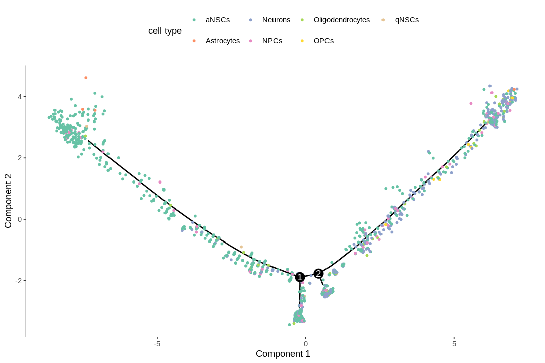
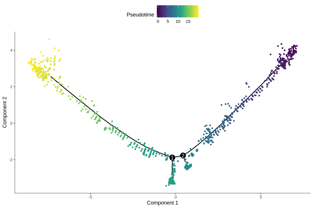
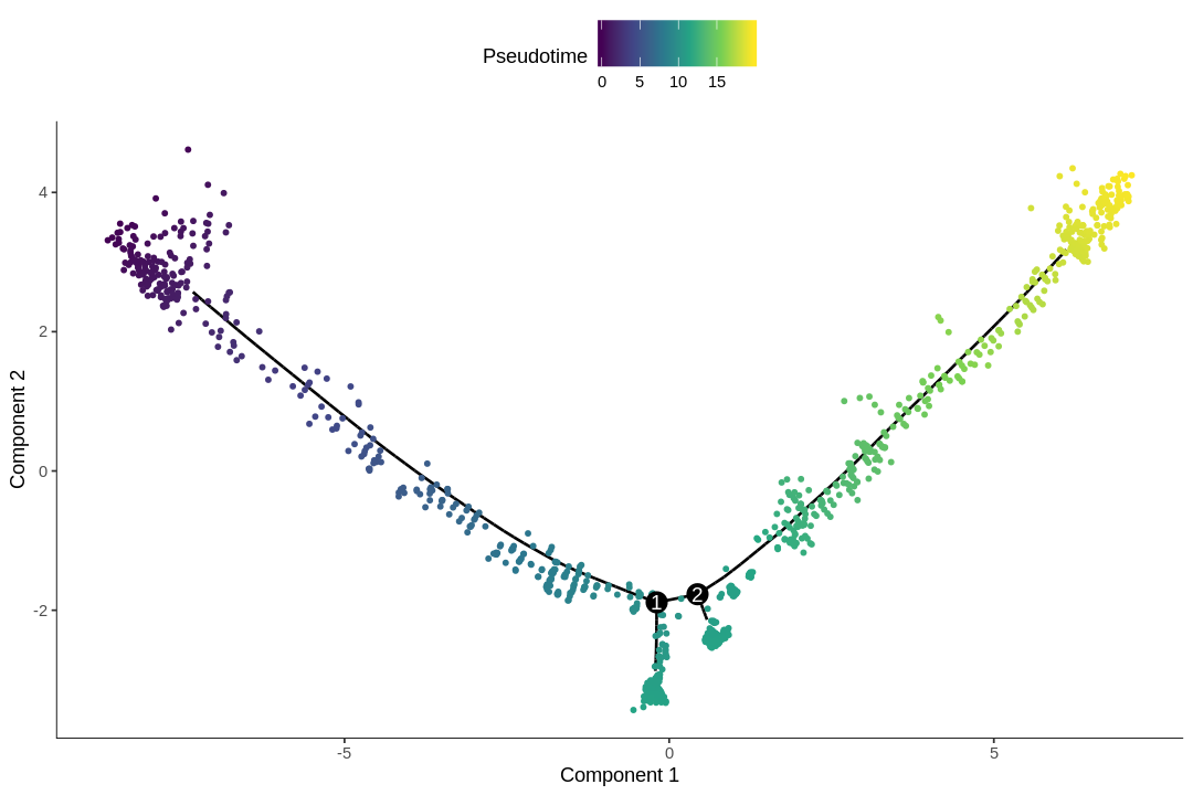
Here Monocle 2 will first project the data to 2 dimensions with DDRTree, and then do trajectory inference (orderCells).

1
2
cds <- reduceDimension(cds, max_components = 2, method = 'DDRTree')
cds <- orderCells(cds)

See what the trajectory looks like. This projection is DDRTree.

1
2
plot_cell_trajectory(cds, color_by = "cell_type", cell_size = 1) +
  scale_color_brewer(name = "cell type", type = "qual", palette = "Set2")

png

In the kallisto | bustools paper, I used slingshot for pseudotime analysis (Supplementary Figure 6.5) of this dataset, and found two neuronal end points. The result from Monocle 2 here also shows two main branches. Also, as expected, the stem cells are at the very beginning of the trajectory.

1
2
plot_cell_trajectory(cds, color_by = "Pseudotime", cell_size = 1) +
  scale_color_viridis_c()

png

The pseudotime values are inverted.

1
2
3
cds <- orderCells(cds, reverse = TRUE)
plot_cell_trajectory(cds, color_by = "Pseudotime", cell_size = 1) +
  scale_color_viridis_c()

png

Monocle 2 can also be used to find genes differentially expressed along the pseudotime trajectory and clusters of such genes. See David Tang's excellent Monocle 2 tutorial for how to use these functionalities.