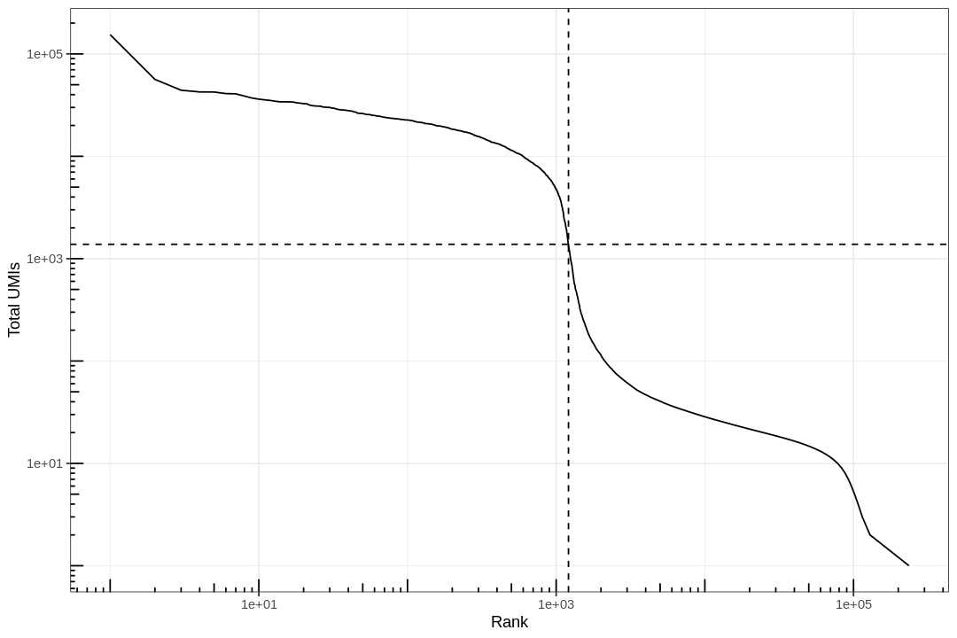
#' Knee plot for filtering empty droplets#' #' Visualizes the inflection point to filter empty droplets. This function plots #' different datasets with a different color. Facets can be added after calling#' this function with `facet_*` functions.#' #' @param bc_rank A `DataFrame` output from `DropletUtil::barcodeRanks`.#' @return A ggplot2 object.knee_plot<-function(bc_rank){knee_plt<-tibble(rank=bc_rank[["rank"]],total=bc_rank[["total"]])%>%distinct()%>%dplyr::filter(total>0)annot<-tibble(inflection=metadata(bc_rank)[["inflection"]],rank_cutoff=max(bc_rank$rank[bc_rank$total>metadata(bc_rank)[["inflection"]]]))p<-ggplot(knee_plt,aes(rank,total))+geom_line()+geom_hline(aes(yintercept=inflection),data=annot,linetype=2)+geom_vline(aes(xintercept=rank_cutoff),data=annot,linetype=2)+scale_x_log10()+scale_y_log10()+annotation_logticks()+labs(x="Rank",y="Total UMIs")return(p)}
Usingtemporarycache/tmp/Rtmp3ZgCkF/BiocFileCachesnapshotDate():2019-10-22Usingtemporarycache/tmp/Rtmp3ZgCkF/BiocFileCachesee?SingleRandbrowseVignettes('SingleR')fordocumentationUsingtemporarycache/tmp/Rtmp3ZgCkF/BiocFileCacheUsingtemporarycache/tmp/Rtmp3ZgCkF/BiocFileCacheUsingtemporarycache/tmp/Rtmp3ZgCkF/BiocFileCacheloadingfromcacheUsingtemporarycache/tmp/Rtmp3ZgCkF/BiocFileCacheUsingtemporarycache/tmp/Rtmp3ZgCkF/BiocFileCacheUsingtemporarycache/tmp/Rtmp3ZgCkF/BiocFileCachesee?SingleRandbrowseVignettes('SingleR')fordocumentationUsingtemporarycache/tmp/Rtmp3ZgCkF/BiocFileCacheUsingtemporarycache/tmp/Rtmp3ZgCkF/BiocFileCacheUsingtemporarycache/tmp/Rtmp3ZgCkF/BiocFileCacheloadingfromcacheUsingtemporarycache/tmp/Rtmp3ZgCkF/BiocFileCacheUsingtemporarycache/tmp/Rtmp3ZgCkF/BiocFileCacheUsingtemporarycache/tmp/Rtmp3ZgCkF/BiocFileCacheUsingtemporarycache/tmp/Rtmp3ZgCkF/BiocFileCachesnapshotDate():2019-10-29Usingtemporarycache/tmp/Rtmp3ZgCkF/BiocFileCacheUsingtemporarycache/tmp/Rtmp3ZgCkF/BiocFileCacheUsingtemporarycache/tmp/Rtmp3ZgCkF/BiocFileCacheUsingtemporarycache/tmp/Rtmp3ZgCkF/BiocFileCacheloadingfromcacheUsingtemporarycache/tmp/Rtmp3ZgCkF/BiocFileCacheUsingtemporarycache/tmp/Rtmp3ZgCkF/BiocFileCacheUsingtemporarycache/tmp/Rtmp3ZgCkF/BiocFileCacheWarningmessage:"Unable to map 2180 of 21214 requested IDs."
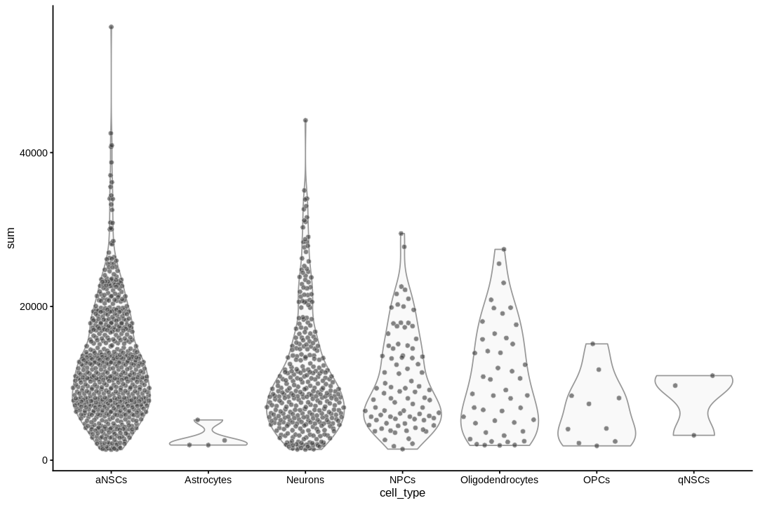
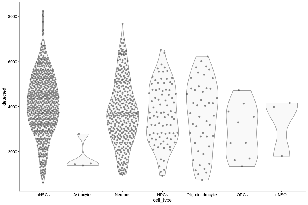
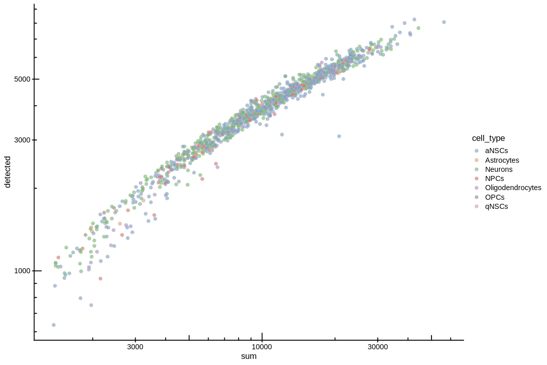
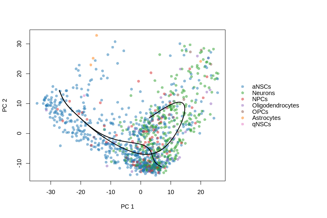
inds<-annots$pruned.labels%in%c("NPCs","Neurons","OPCs","Oligodendrocytes","qNSCs","aNSCs","Astrocytes","Ependymal")# Only keep these cell typescells_use<-row.names(annots)[inds]sce<-sce[,cells_use]sce$cell_type<-annots$pruned.labels[inds]
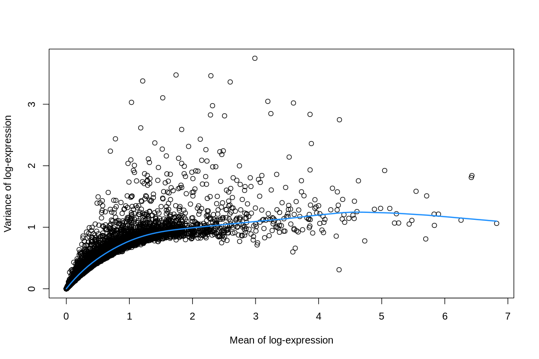
# Adapted from https://osca.bioconductor.org/feature-selection.html#feature-selectionplot(fit_pbmc$mean,fit_pbmc$var,xlab="Mean of log-expression",ylab="Variance of log-expression")curve(fit_pbmc$trend(x),col="dodgerblue",add=TRUE,lwd=2)
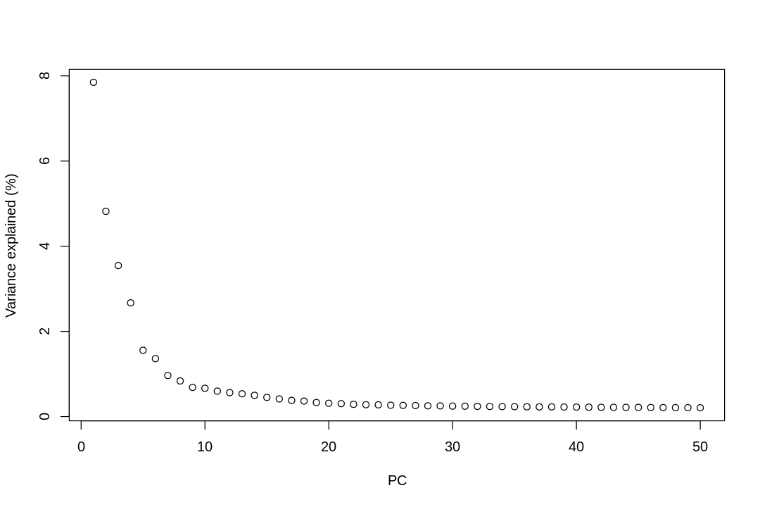
# Percentage of variance explained is tucked away in the attributes.percent.var<-attr(reducedDim(sce),"percentVar")plot(percent.var,xlab="PC",ylab="Variance explained (%)")
The y axis is percentage of variance explained by the PC, or the eigenvalues of the covariance matrix.
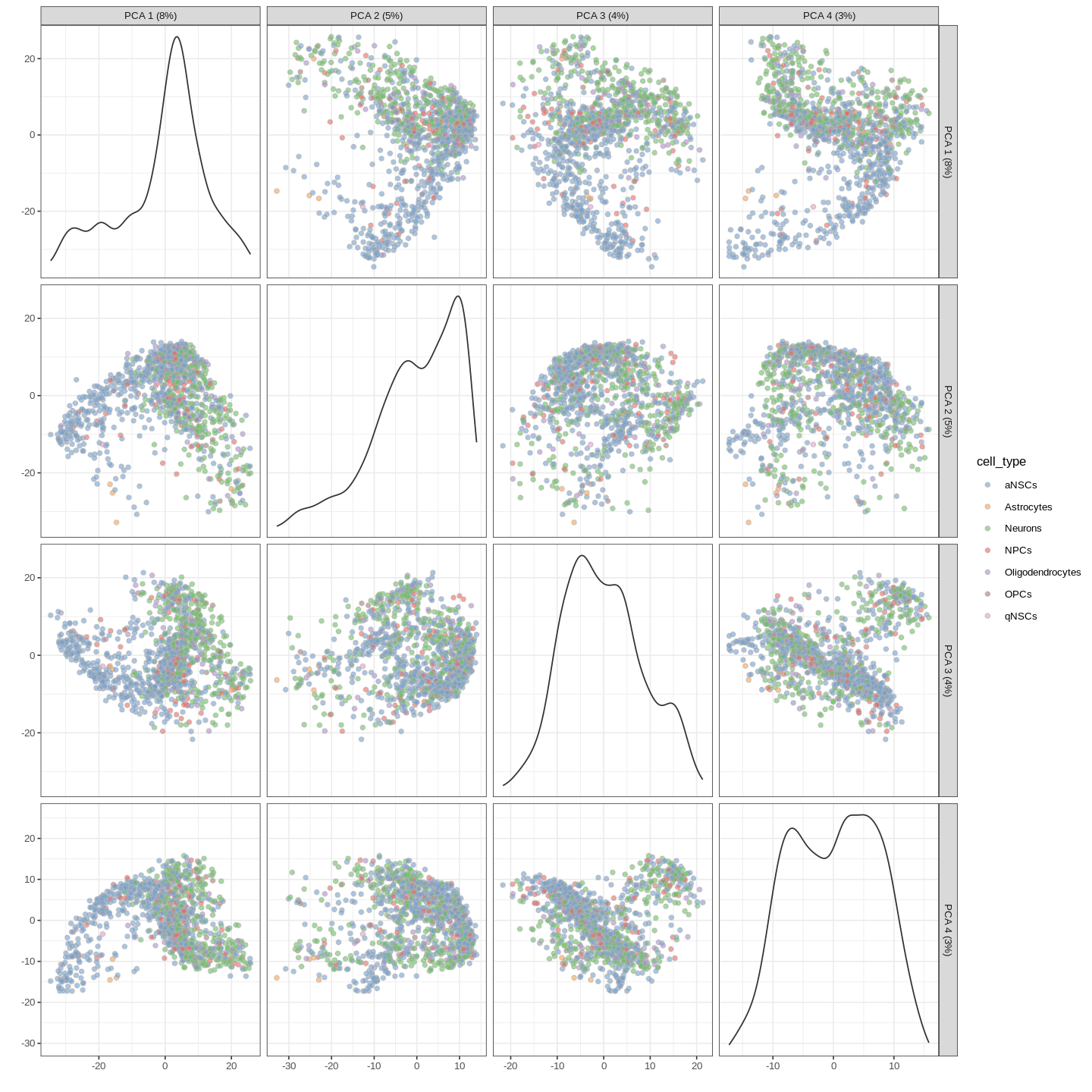
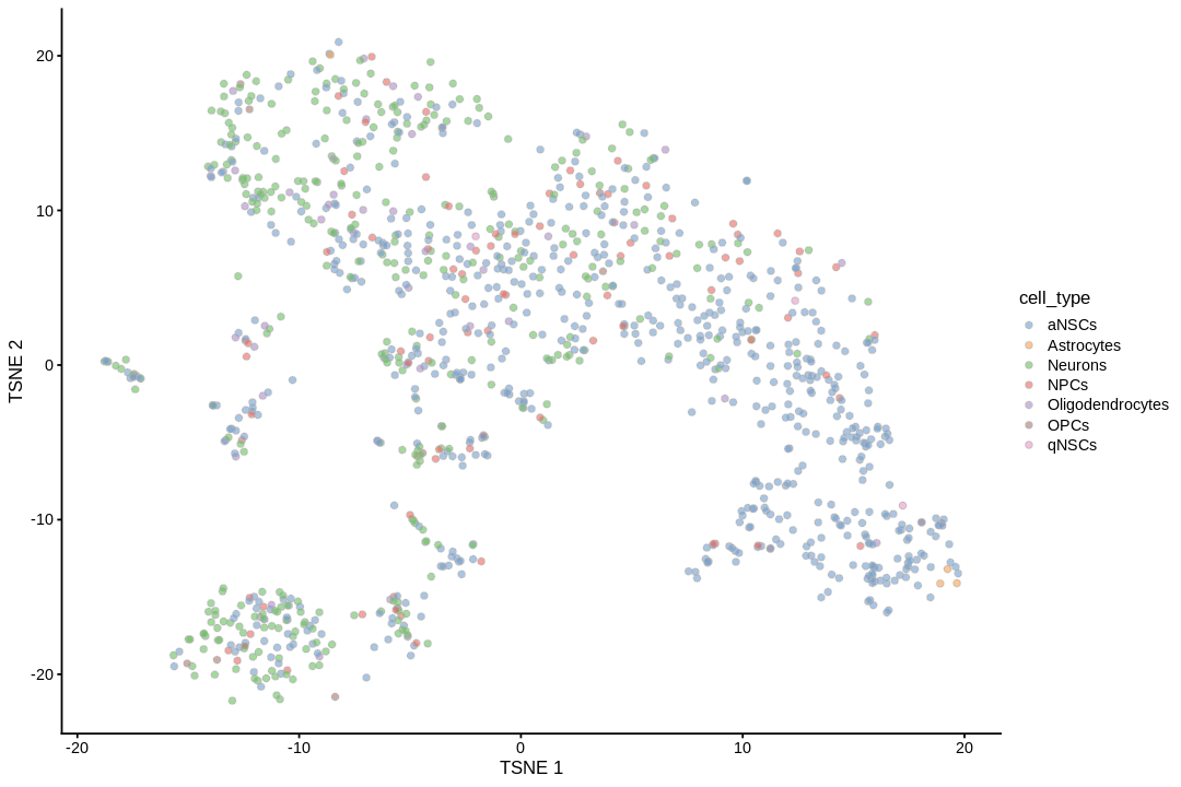
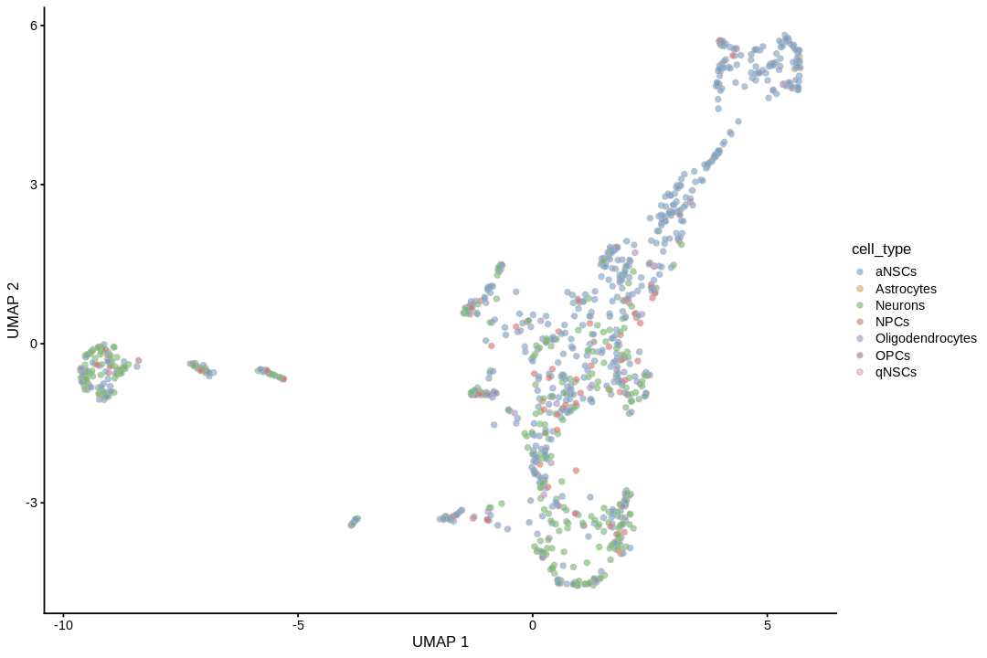
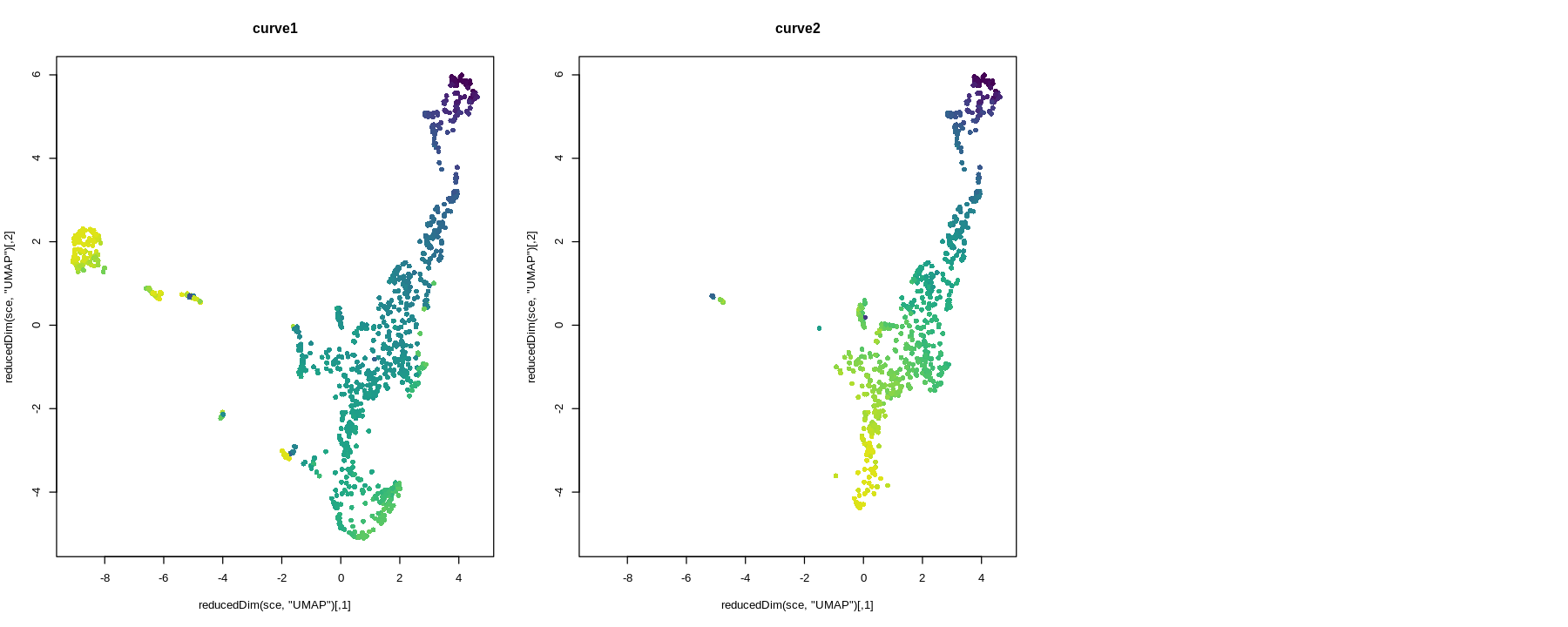
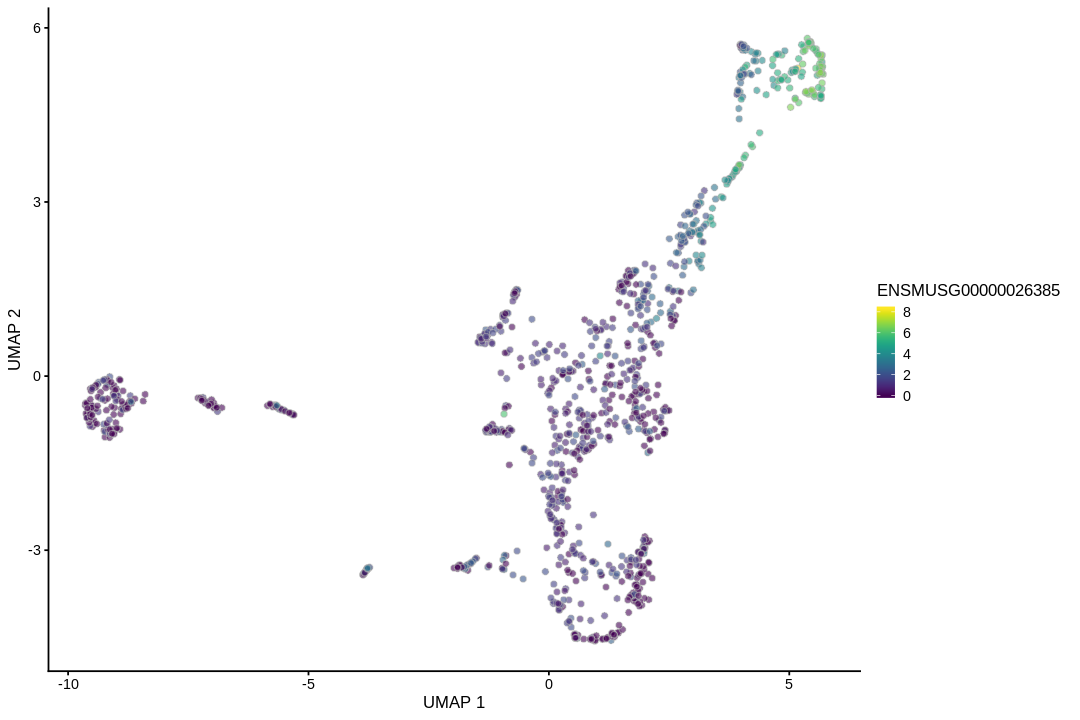
UMAP can better preserve pairwise distance of cells than tSNE and can better separate cell populations than the first 2 PCs of PCA (Becht et al. 2018), so the TI will be visualized on UMAP rather than tSNE or PCA.
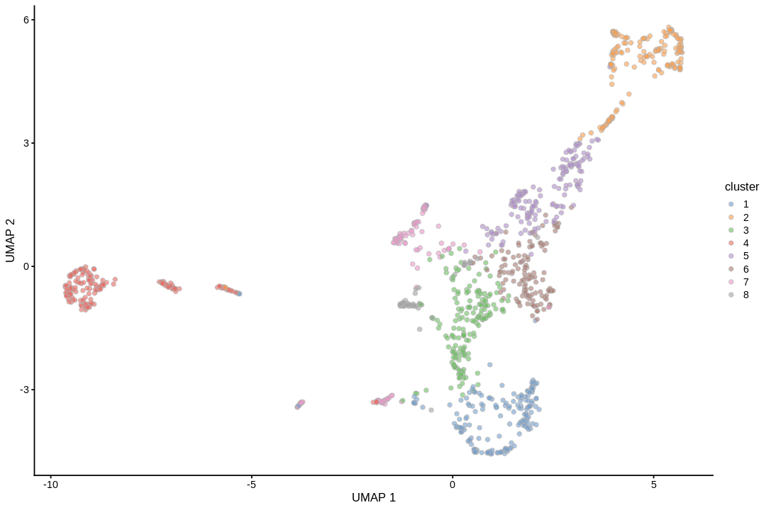
Cell type annotation with SingleR requires a reference with bulk RNA seq data for isolated known cell types. The reference used for cell type annotation here does not differentiate between different types of neural progenitor cells; clustering can further partition the neural progenitor cells. Furthermore, slingshot is based on cluster-wise minimum spanning tree, so finding a good clustering is important to good trajectory inference with slingshot. The clustering algorithm used here is Leiden, which is an improvement over the commonly used Louvain; Leiden communities are guaranteed to be well-connected, while Louvain can lead to poorly connected communities.
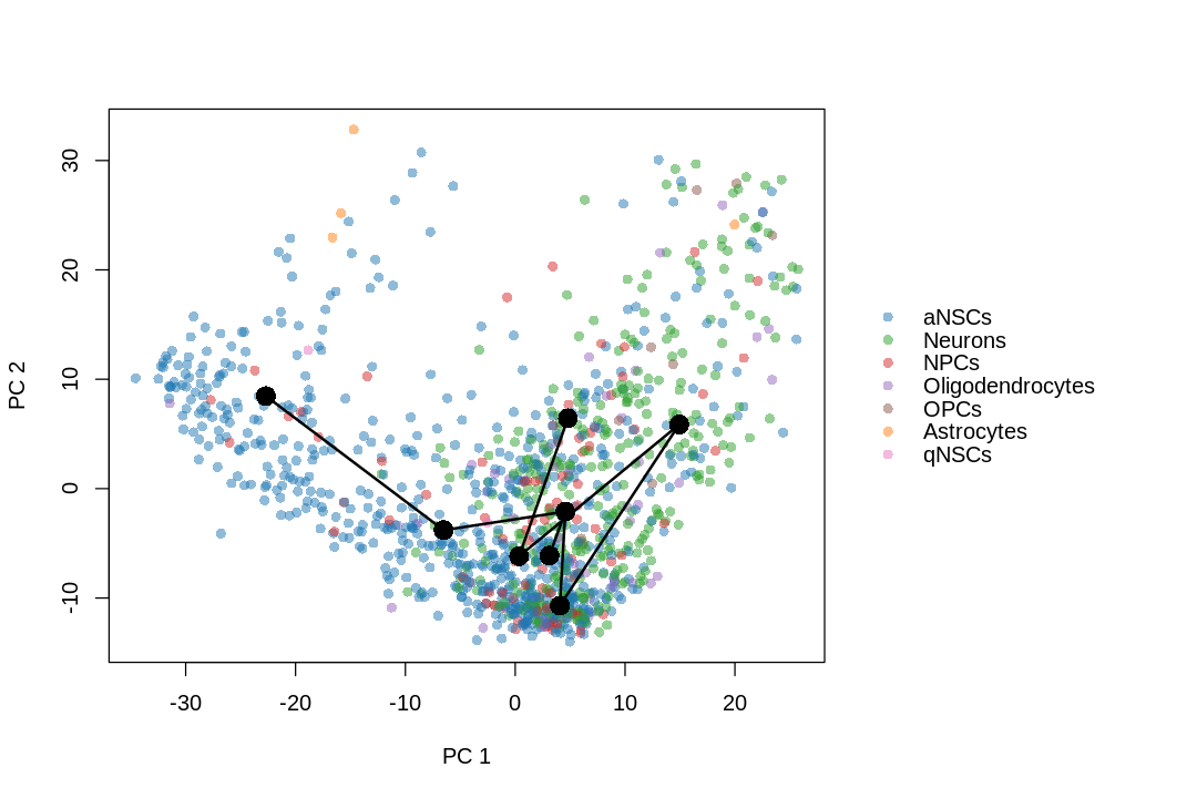
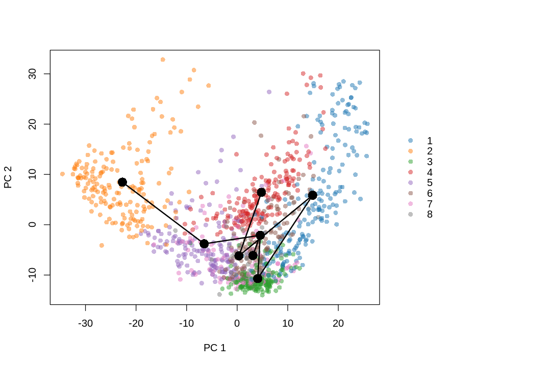
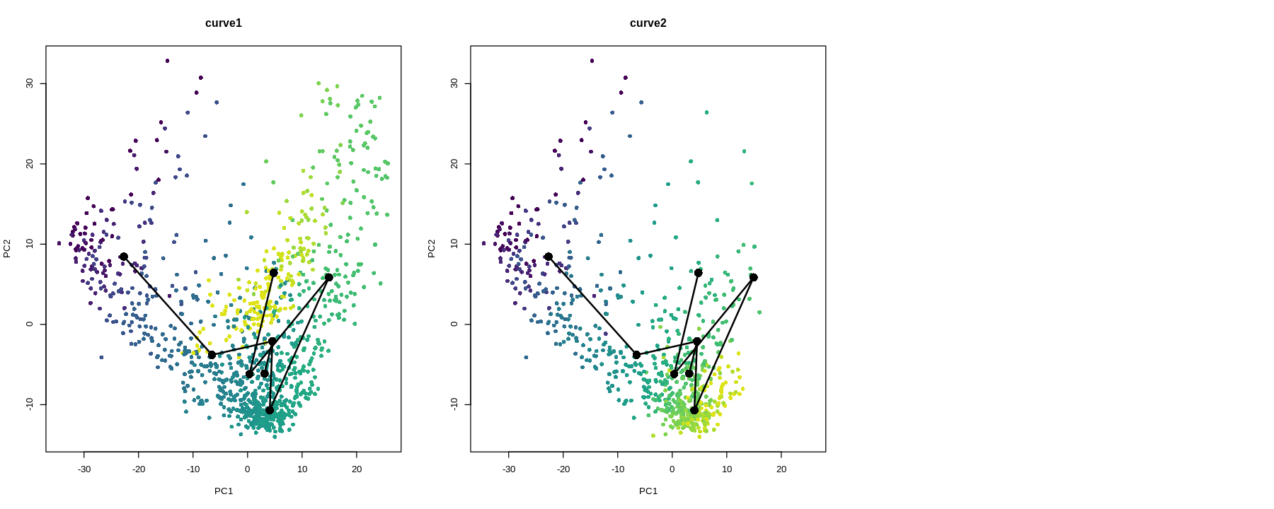
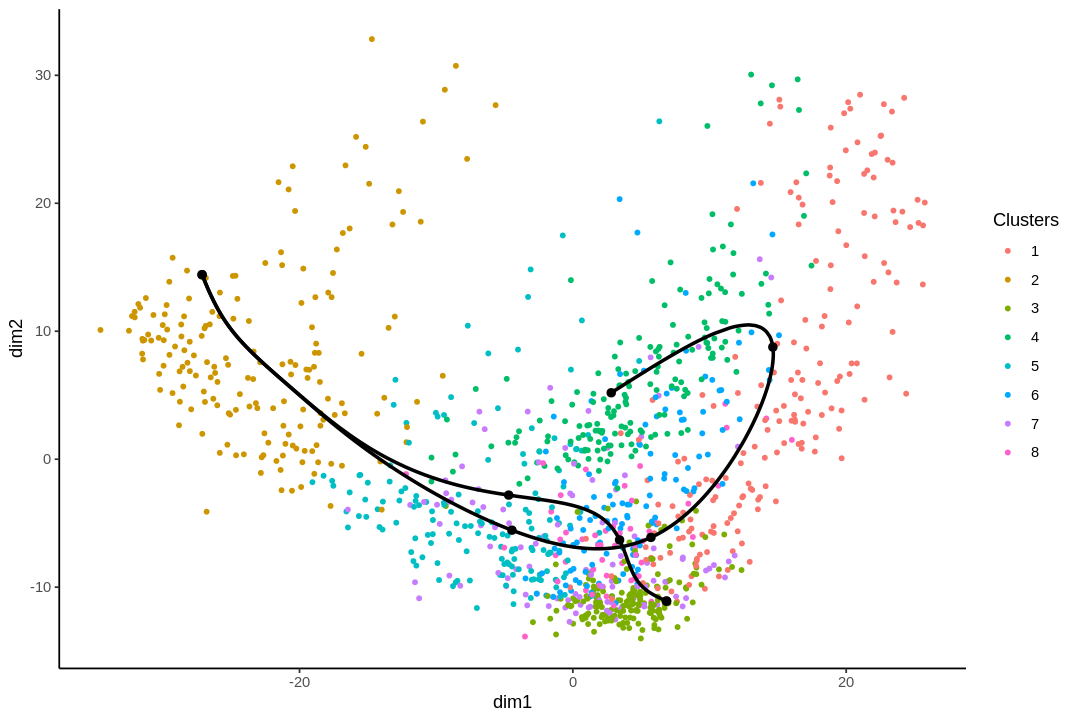
While the slingshot vignette uses SingleCellExperiment, slingshot can also take a matrix of cell embeddings in reduced dimension as input. We can optionally specify the cluster to start or end the trajectory based on biological knowledge. Here, since quiescent neural stem cells are in cluster 4, the starting cluster would be 4 near the top left of the previous plot.
I no longer consider doing trajectory inference on UMAP a good idea, due to distortions introduced by UMAP. See this paper for the extent non-linear dimension reduction methods distort the data. The latent dimension of the data is most likely far more than 2 or 3 dimensions, so forcing it down to 2 or 3 dimensions are bound to introduce distortions, just like how projecting the spherical surface of the Earth to 2 dimensions in maps introduces distortions. Furthermore, after the projection, some trajectories are no longer topologically feasible. For instance, imagine a stream coming out of the hole of a doughnut in 3D. This is not possible in 2D, so when that structure is projected to 2D, part of the stream may become buried in the middle of the doughnut, or the doughnut may be broken to allow the stream through, or part of the steam will be intermixed with part of the doughnut though they shouldn't. I recommend using a larger number of principal components instead, but in that case, the lineages and principal curves can't be visualized (we can plot the curves within a 2 dimensional subspace, such as the first 2 PCs, but that usually looks like abstract art and isn't informative about the lineages).
Unfortunately, slingshot does not natively support ggplot2. So this is a function that assigns colors to each cell in base R graphics.
1 2 3 4 5 6 7 8 91011121314151617
#' Assign a color to each cell based on some value#' #' @param cell_vars Vector indicating the value of a variable associated with cells.#' @param pal_fun Palette function that returns a vector of hex colors, whose#' argument is the length of such a vector.#' @param ... Extra arguments for pal_fun.#' @return A vector of hex colors with one entry for each cell.cell_pal<-function(cell_vars,pal_fun,...){if (is.numeric(cell_vars)){pal<-pal_fun(100,...)return(pal[cut(cell_vars,breaks=100)])}else{categories<-sort(unique(cell_vars))pal<-setNames(pal_fun(length(categories),...),categories)return(pal[cell_vars])}}
We need color palettes for both cell types and Leiden clusters. These would be the same colors seen in the Seurat plots.