Introduction to single-cell RNA-seq II: getting started with analysis
This notebook demonstrates pre-processing and basic analysis of the mouse retinal cells GSE126783 dataset from Koren et al., 2019. Following pre-processing using kallisto and bustools and basic QC, the notebook demonstrates some initial analysis. The approximate running time of the notebook is 12 minutes.
The notebook was written by Kyung Hoi (Joseph) Min, Lambda Lu, A. Sina Booeshaghi and Lior Pachter. If you use the methods in this notebook for your analysis please cite the following publications which describe the tools used in the notebook, as well as specific methods they run (these are cited inline in the notebook):
Melsted, P., Booeshaghi, A.S. et al. Modular and efficient pre-processing of single-cell RNA-seq. bioRxiv (2019). doi:10.1101/673285
McCarthy, D.J., Campbell, K.R., Lun, A.T. and Wills, Q.F. Scater: pre-processing, quality control, normalization and visualization of single-cell RNA-seq data in R (2017). doi.org/10.1093/bioinformatics/btw777
A Python notebook implementing the same analysis is available here. See the kallistobus.tools tutorials site for additional notebooks demonstrating other analyses.
# Slightly modified from BUSpaRse, just to avoid installing a few dependencies not used hereread_count_output<-function(dir,name){dir<-normalizePath(dir,mustWork=TRUE)m<-readMM(paste0(dir,"/",name,".mtx"))m<-Matrix::t(m)m<-as(m,"dgCMatrix")# The matrix read has cells in rowsge<-".genes.txt"genes<-readLines(file(paste0(dir,"/",name,ge)))barcodes<-readLines(file(paste0(dir,"/",name,".barcodes.txt")))colnames(m)<-barcodesrownames(m)<-genesreturn(m)}
The following command will generate an RNA count matrix of cells (rows) by genes (columns) in H5AD format, which is a binary format used to store Anndata objects. Notice that this requires providing the index and transcript-to-gene mapping downloaded in the previous step to the -i and -g arguments respectively. Also, since the reads were generated with the 10x Genomics Chromium Single Cell v2 Chemistry, the -x 10xv2 argument is used. To view other supported technologies, run kb --list.
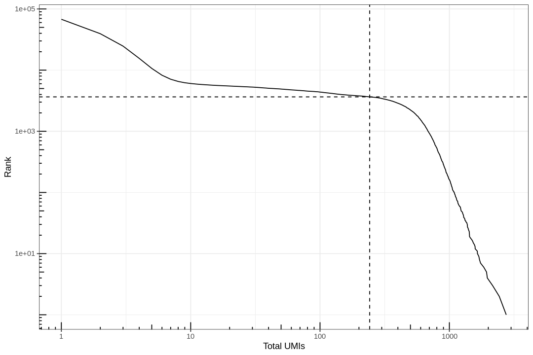
Most barcodes in the matrix correspond to empty droplets. A common way to determine which barcodes are empty droplets and which are real cells is to plot the rank of total UMI counts of each barcode against the total UMI count itself, which is commonly called knee plot. The inflection point in that plot, signifying a change in state, is used as a cutoff for total UMI counts; barcodes below that cutoff are deemed empty droplets and removed.
In this plot cells are ordered by the number of UMI counts associated to them (shown on the x-axis), and the fraction of droplets with at least that number of cells is shown on the y-axis:
#' Knee plot for filtering empty droplets#' #' Visualizes the inflection point to filter empty droplets. This function plots #' different datasets with a different color. Facets can be added after calling#' this function with `facet_*` functions. Will be added to the next release#' version of BUSpaRse.#' #' @param bc_rank A `DataFrame` output from `DropletUtil::barcodeRanks`.#' @return A ggplot2 object.knee_plot<-function(bc_rank){knee_plt<-tibble(rank=bc_rank[["rank"]],total=bc_rank[["total"]])%>%distinct()%>%dplyr::filter(total>0)annot<-tibble(inflection=metadata(bc_rank)[["inflection"]],rank_cutoff=max(bc_rank$rank[bc_rank$total>metadata(bc_rank)[["inflection"]]]))p<-ggplot(knee_plt,aes(total,rank))+geom_line()+geom_hline(aes(yintercept=rank_cutoff),data=annot,linetype=2)+geom_vline(aes(xintercept=inflection),data=annot,linetype=2)+scale_x_log10()+scale_y_log10()+annotation_logticks()+labs(y="Rank",x="Total UMIs")return(p)}
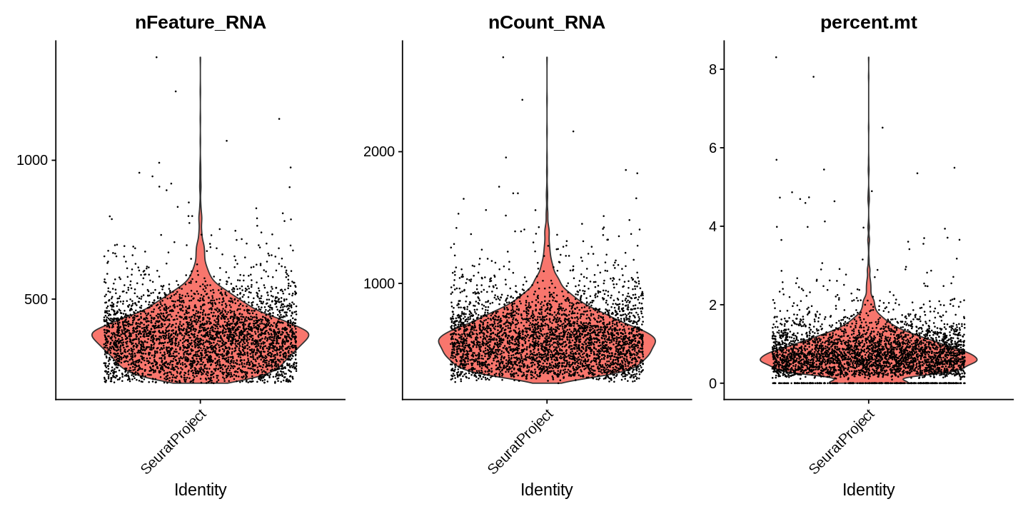
# Visualize QC metrics as a violin plotoptions(repr.plot.width=12,repr.plot.height=6)VlnPlot(seu,features=c("nFeature_RNA","nCount_RNA","percent.mt"),ncol=3,pt.size=0.1)
12345678
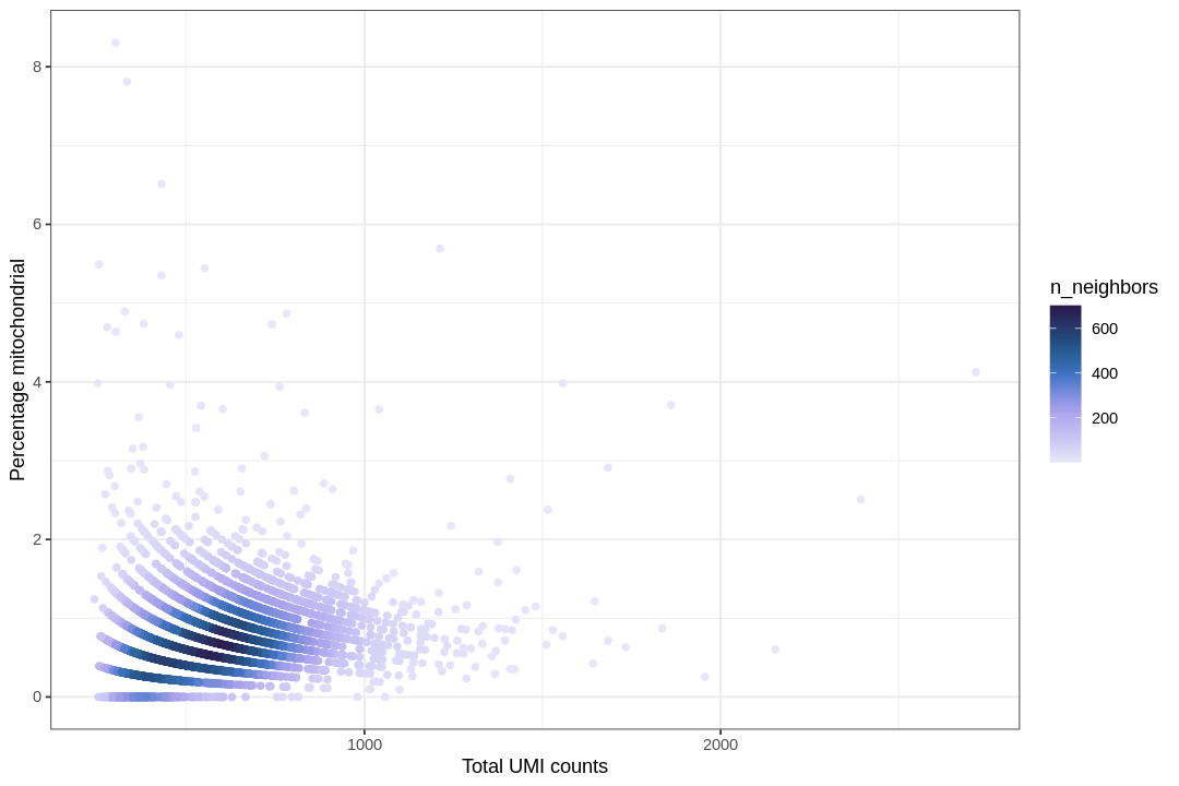
options(repr.plot.width=9,repr.plot.height=6)ggplot(seu@meta.data,aes(nCount_RNA,nFeature_RNA))+geom_hex(bins=100)+scale_fill_scico(palette="devon",direction=-1,end=0.9)+scale_x_log10(breaks=breaks_log(12))+scale_y_log10(breaks=breaks_log(12))+annotation_logticks()+labs(x="Total UMI counts",y="Number of genes detected")+theme(panel.grid.minor=element_blank())
The color shows density of points, as the density is not apparent when many points are stacked on top of each other. Cells with high percentage of mitochondrially encoded transcripts are often removed in QC, as those are likely to be low quality cells. If a cell is lysed in sample preparation, transcripts in the mitochondria are less likely to be lost than transcripts in the cytoplasm due to the double membrane of the mitochondria, so cells that lysed tend to have a higher percentage of mitochondrially encoded transcripts.
We filter cells with more than 3% mitochondrial content based on the plot above.
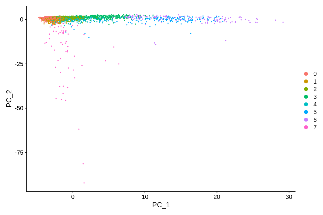
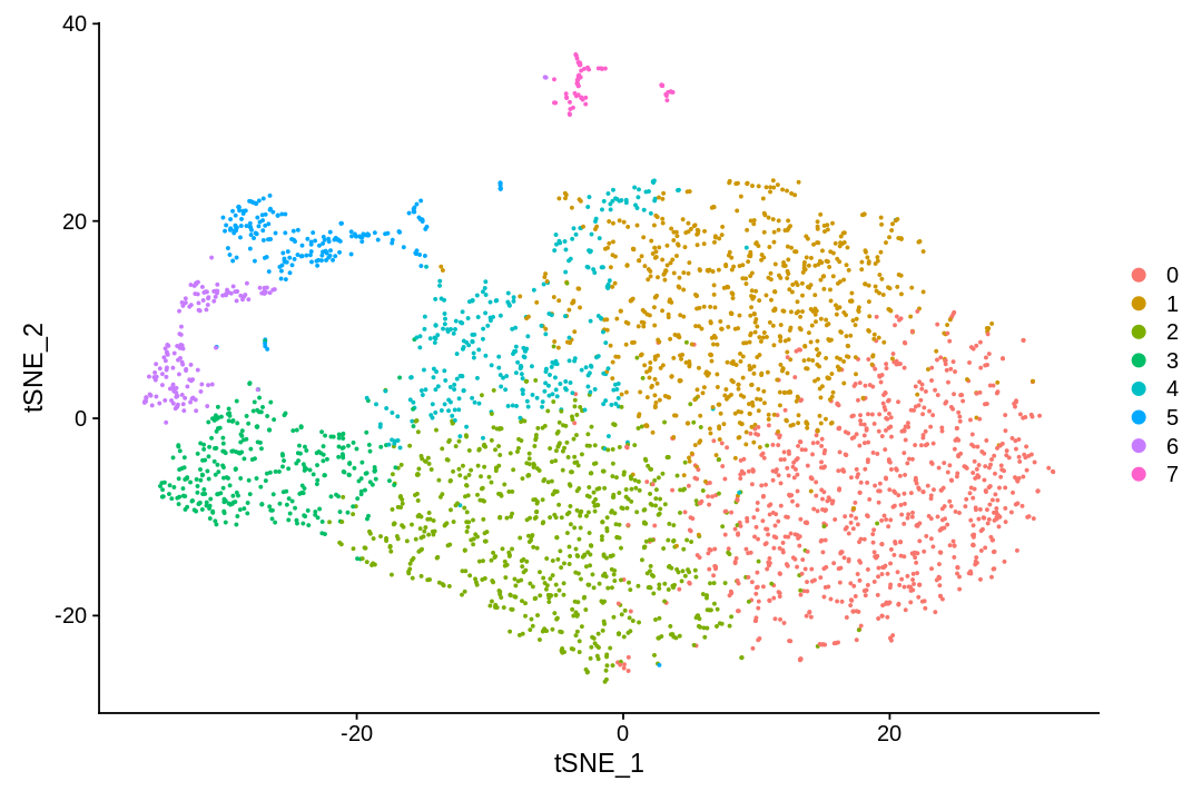
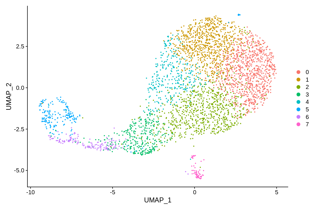
There are many algorithms for clustering cells, and while they have been compared in detail in various benchmarks (see e.g., Duo et al. 2018), there is no univerally agreed upon method. Here we demonstrate clustering using Louvain clustering, which is a popular method for clustering single-cell RNA-seq data. The method was published in
Blondel, Vincent D; Guillaume, Jean-Loup; Lambiotte, Renaud; Lefebvre, Etienne (9 October 2008). "Fast unfolding of communities in large networks". Journal of Statistical Mechanics: Theory and Experiment. 2008 (10): P10008.
UMAP (UMAP: Uniform Manifold Approximation and Projection for Dimension Reduction) is a manifold learning technique that can also be used to visualize cells. It was published in:
McInnes, Leland, John Healy, and James Melville. "Umap: Uniform manifold approximation and projection for dimension reduction." arXiv preprint arXiv:1802.03426 (2018).
This notebook has demonstrated visualization of cells following pre-processing of single-cell RNA-seq data.
1
Sys.time()-start_time
Time difference of 38.41409 mins
Installing packages took about 26 minutes, which is a drawback of Rcpp. The QC and analysis post-installation takes about 10 minutes from reads to results. This includes downloading the data, filtering, clustering and visualization.